Section 4 Data treatment
4.1 Joining a layer data
Another frequent task before executing spatial analysis with QGIS is to join an attribute table to a layer.
To illustrate this task, we refer to the stations_rsqa.shp file generated in section 1 and the file pollutants_average_12_31_2019_13H.csv file. When we load the shapefile into QGIS we identify that this layer only contains information on the identification and location of stations that compose the Air Quality Monitoring Network (RSQA).
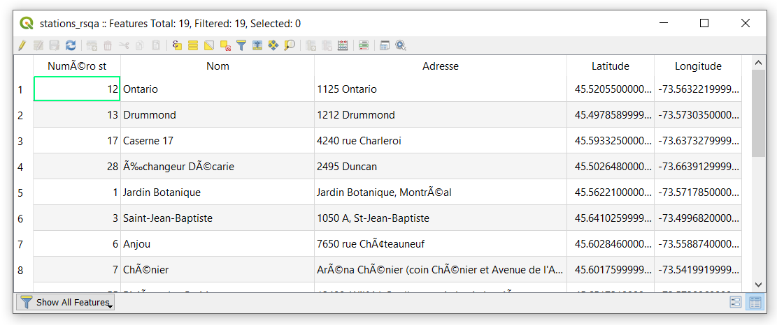
Figure 4.1: Attribute table of stations
We realize another problem, the name (nom) and the address of the stations are not correctly displayed. In order to fix it, right-click on the name of the layer, and select properties. A window will pop up. Go to Source and change the Data Source Encoding to UTF-8. Finally, click on Apply to accept the changes.
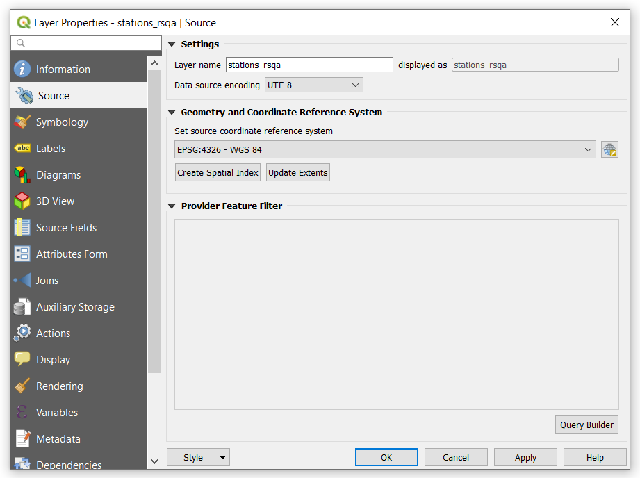
Figure 4.2: Changing encoding
Now, import the pollutants_average_12_31_2019_13H.csv file. One kick method is to drag and drop the file from the file into QGIS. This works fine for this file; however, you also can use Add Delimited Text Layer to have more control on the importation.
The pollutants_average_12_31_2019_13H.csv file reports the average concentration of criteria pollutants from December 23, 2013, at 12h. The units of concentration are indicated in the following table.
| Pollutant | Unit |
|---|---|
| CO | ppm |
| H2S | ppb |
| NO | ppb |
| NO2 | ppb |
| SO2 | \(\mu g/m^3\) |
| PM10 | \(\mu g/m^3\) |
| PM2.5 | \(\mu g/m^3\) |
| O3 | ppb |
In order to join the pollutants_average_12_31_2019_13H attribute table to the stations_rsqa layer, follow these steps:
- Right-click on the name of
stations_rsqalayer, select Properties, then Joins from the dialog window.
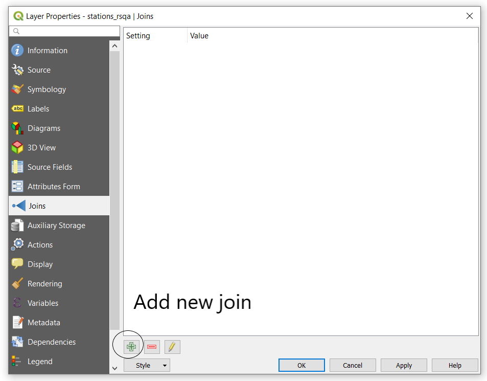
Figure 4.3: Layer properties window
- Click on the green + sign. The following window will pop up:
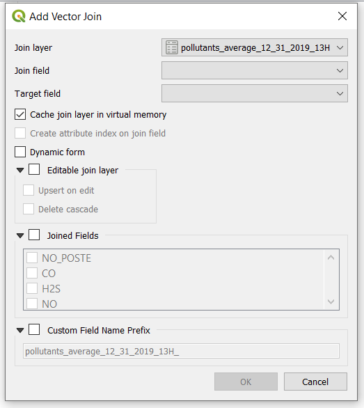
Figure 4.4: Joining a layer table
In this case, since we have imported only one attribute table, QGIS has already selected the Join layer.
Specify the Join field and the Target field, which correspond to the keys that relate the shapefile layer and the data layer. In this example, NO_POSTE is the identifier of the stations in the data layer and Numéro st is the identifier of the stations in the shapefile layer. Furthermore, it is possible to select the fields that will be joined, and the prefix that will be used. Since there are no repeated columns, we just deleted the default prefix, which corresponds to the name of the layer.
Click on OK, then on Apply to finish the joining.
To verify if the join has worked, you can open the attribute table of the shapefile. To make this change permanent, you need to export the layer. After the join, the layer was exported as
stations_rsqa_12_31_2013.shp.
4.2 Cleaning up the attribute table
Sometimes, data imported into QGIS is not in the correct format, the name of columns is not self-explanatory, or we simply want to discard the columns that will not be used during the task in hand.
The Refactor fields algorithm simplifies removing, renaming and converting the format of dbf tables in QGIS. This algorithm ca be accessed through the Processing Toolbox. The use of Refactor fields is illustrated with the stations_rsqa_12_31_2013.shp file that was generated in the previous section.
- Import
stations_rsqa_12_31_2013.shpfile - Launch the Refactor field. It will detect the available layer in the current project. In this window we can identify the name of columns, the type of information they store, their length and precision. The columns corresponding to concentrations, such as CO, H2S, and NO, are currently stored as text (data type is string). This is not convenient, since we cannot do arithmetic with text. Furthermore, we may want to change the name of Numéro st field for Station.
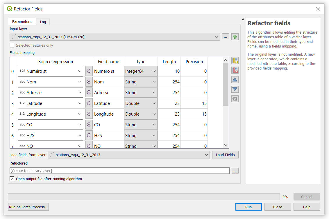
Figure 4.5: Refactor field window
- We change the name of the first three columns according to the following figure, and the type of columns corresponding to concentrations was set as Double (real number) with a length of 23 and a precision of 3. Click on Run to generate a new layer.
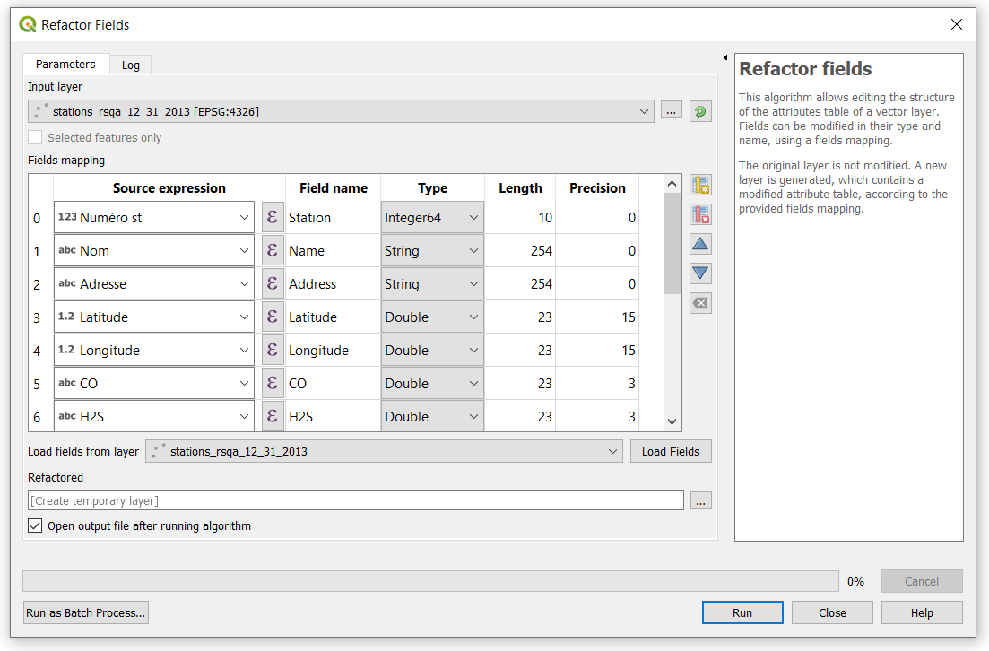
Figure 4.6: Using the refactor field algorithm
- The generated layer is named by default Refactored, of course, you can change its name at your convenience.
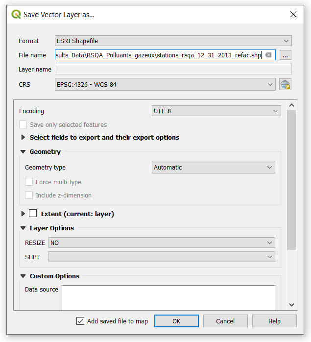
Figure 4.7: Saving the refactored layer